Smart classification using Bayesian monads in Haskell

(Refactoring Probability Distributions: part 1, part 2, part 3, part 4)

The world is full of messy classification problems:

“Is this order fraudulent?”
“It this e-mail a spam?”
“What blog posts would Rachel find interesting?”
“Which intranet documents is Sam looking for?”

In each case, we want to classify something: Orders are either valid or fraudulent, messages are either spam or non-spam, blog posts are either interesting or boring. Unfortunately, most software is terrible at making these distinctions. For example, why can’t my RSS reader go out and track down the 10 most interesting blog posts every day?

Some software, however, can make these distinctions. Google figures out when I want to watch a movie, and shows me specialized search results. And most e-mail clients can identify spam with over 99% accuracy. But the vast majority of software is dumb, incapable of dealing with the messy dilemmas posed by the real world.

So where can we learn to improve our software?

Outside of Google’s shroud of secrecy, the most successful classifiers are spam filters. And most modern spam filters are inspired by Paul Graham’s essay A Plan for Spam.

So let’s go back to the source, and see what we can learn. As it turns out, we can formulate a lot of the ideas in A Plan for Spam in a straightforward fashion using a Bayesian monad.

Functions from distributions to distributions

Let’s begin with spam filtering. By convention, we divide messages into “spam” and “ham”, where “ham” is the stuff we want to read.

data MsgType = Spam | Ham
  deriving (Show, Eq, Enum, Bounded)

Let’s assume that we’ve just received a new e-mail. Without even looking at it, we know there’s a certain chance that it’s a spam. This gives us something called a “prior distribution” over MsgType.

> bayes msgTypePrior
[Perhaps Spam 64.2%, Perhaps Ham 35.8%]

But what if we know that the first word of the message is “free”? We can use that information to calculate a new distribution.

> bayes (hasWord "free" msgTypePrior)
[Perhaps Spam 90.5%, Perhaps Ham 9.5%]

The function hasWord takes a string and a probability distribution, and uses them to calculate a new probability distribution:

hasWord :: String -> FDist' MsgType ->
           FDist' MsgType
hasWord word prior = do
  msgType <- prior
  wordPresent <-
    wordPresentDist msgType word
  condition wordPresent
  return msgType

This code is based on the Bayesian monad from part 3. As before, the “<-” operator selects a single item from a probability distribution, and “condition” asserts that an expression is true. The actual Bayesian inference happens behind the scenes (handy, that).

If we have multiple pieces of evidence, we can apply them one at a time. Each piece of evidence will update the probability distribution produced by the previous step:

hasWords []     prior = prior
hasWords (w:ws) prior = do
  hasWord w (hasWords ws prior)

The final distribution will combine everything we know:

> bayes (hasWords ["free","bayes"] msgTypePrior)
[Perhaps Spam 34.7%, Perhaps Ham 65.3%]

This technique is known as the naive Bayes classifier. Looked at from the right angle, it’s surprisingly simple.

(Of course, the naive Bayes classifier assumes that all of our evidence is independent. In theory, this is a pretty big assumption. In practice, it works better than you might think.)

But this still leaves us with a lot of questions: How do we keep track of our different classifiers? How do we decide which ones to apply? And do we need to fudge the numbers to get reasonable results?

In the following sections, I’ll walk through various aspects of Paul Graham’s A Plan for Spam, and show how to generalize it. If you want to follow along, you can download the code using Darcs:

darcs get http://www.randomhacks.net/darcs/probability

The basic implementation

The first version of our library will be very simple. First, we’ll need to keep track of how many spams and hams we’ve seen, and how often each word appears in spams and hams. We’ll store these numbers in lists, in case we later decide to add a third type of message:

-- [Spam count, ham count]
msgCounts = [102, 57]

-- Number of spams and hams containing
-- each word.
wordCountTable =
  M.fromList [("free", [57, 6]),
              -- Lots of words...
              ("bayes", [1, 10]),
              ("monad", [0, 22])]

-- This is basically a Haskell
-- version of 'ys[x]'.
entryFor :: Enum a => a -> [b] -> b
entryFor x ys = ys !! fromEnum x

Using this data, we can easily calculate our prior distribution:

msgTypePrior :: Dist d => d MsgType
msgTypePrior =
  weighted (zip [Spam,Ham] msgCounts)

We can also calculate what percentage of each type of message contains a specific word. (Note that we represent the percentage as a Boolean distribution: “There’s a 75% chance of true, and a 25% chance of false.”)

wordPresentDist msgType word =
    boolDist (Prob (n/total))
  where wordCounts = findWordCounts word
        n     = entryFor msgType wordCounts
        total = entryFor msgType msgCounts

boolDist :: Prob -> FDist' Bool
boolDist (Prob p) =
    weighted [(True, p), (False, 1-p)]

findWordCounts word =
  M.findWithDefault [0,0] word wordCountTable

From this data, we can answer the question, “Given that an e-mail contains the word ‘bayes’, what’s the chance that it’s a spam?”

> bayes (hasWord "bayes" msgTypePrior)
[Perhaps Spam 9.1%, Perhaps Ham 90.9%]

By itself, this would make a semi-tolerable spam filter. But if we want it to perform well, we’ll need to tweak it.

Deciding which classifiers to use

The first problem: Not all the words in a message will give us useful evidence. In fact, most of the words will bump the prior distribution very slightly in an arbitrary direction. And as Paul Graham discovered, too many of these slight bumps can actually lower the effectiveness of our classifier. We’ll get better results if we only look at the biggest bumps.

Of course, that means we’ll need to “score” each classifier by the size of the bump it produces. First, we’ll need to start with a perfectly flat distribution:

uniformAll :: (Dist d,Enum a,Bounded a) => d a
uniformAll = uniform allValues

allValues :: (Enum a, Bounded a) => [a]
allValues = enumFromTo minBound maxBound

With a two-element type, this gives us a 50/50 split:

> bayes (uniformAll :: FDist' MsgType)
[Perhaps Spam 50.0%, Perhaps Ham 50.0%]

Next, for any function which maps one probability distribution to another, we can calculate a “characteristic” distribution. This measures how much the function bumps the perfectly flat distribution.

characteristic f = f uniformAll

For example, we can calculate the characteristic distribution for the word “free” as follows:

> bayes (characteristic (hasWord "free"))
[Perhaps Spam 84.1%, Perhaps Ham 15.9%]

Now, we could choose to score this distribution the way Paul Graham did, by calculating (0.841 - 0.5) and taking the absolute value. But if we ever want to handle more than two types of messages, we’ll need to do something a bit more elaborate. We could, for example, treat the distributions as vectors, and calculate the distance between them:

score f =
  distance (characteristic f) uniformAll

-- Euclidean distance, minus the final
-- square root (which makes no difference
-- and wastes a lot of cycles).
distance :: (Eq a, Enum a, Bounded a) =>
            FDist' a -> FDist' a -> Double
distance dist1 dist2 =
    sum (map (^2) (zipWith (-) ps1 ps2))
  where ps1 = vectorFromDist dist1
        ps2 = vectorFromDist dist2

vectorFromDist dist =
  map doubleFromProb (probsFromDist dist)

probsFromDist dist =
    map (\x -> (sumProbs . matching x) (bayes dist))
        allValues
  where matching x = filter ((==x) . perhapsValue)
        sumProbs = sum . map perhapsProb

Now that we’ve defined score, we can say things like, “Take the 15 classifiers with the highest scores, and apply those to the message.”

Dealing with 0% and 100%

There’s one serious bug in our code so far: If we’ve seen a word only in spams, but never in hams, then our code will assume that any message containing that word is 100% certain to be a spam. Any other evidence will be ignored, causing weird results.

> let dist = characteristic (hasWord "monad")
> probsFromDist dist
[0.0%,100.0%]

We could fix this by replacing all the zeros in our wordCountTable with some tiny value (a process known a Laplace smoothing). Or we could do what Paul Graham did, and fudge the percentages after we’ve calculated them. Again, this is slightly harder for us, because we’re trying to support more than two types of messages:

adjustedProbsFromDist dist =
  adjustMinimums (probsFromDist dist)

adjustMinimums xs = map (/ total) adjusted
  where adjusted = map (max 0.01) xs
        total = sum adjusted

This gets rid of that nasty 0%:

> adjustedProbsFromDist dist
[1.0%,99.0%]

Applying probabilities directly

Now that we have these nice probability vectors, we’d prefer to use them directly (and not keep calling hasWord). As it turns out, there’s a clever way to cheat here, and still get the right answer:

-- Convert f to a probability vector.
classifierProbs f =
   adjustedProbsFromDist (characteristic f)

-- Apply a probability vector to a prior
-- distribution.
applyProbs probs prior = do
  msgType <- prior
  applyProb (entryFor msgType probs)
  return msgType

We get the same results, regardless of whether we do things the old way:

> bayes (hasWord "free" msgTypePrior)
[Perhaps Spam 90.5%, Perhaps Ham 9.5%]

Or the new way:

> let probs = classifierProbs (hasWord "free")
> bayes (applyProbs probs msgTypePrior)
[Perhaps Spam 90.5%, Perhaps Ham 9.5%]

The trick is in the applyProb, which forks our underlying computation and kills off half the branches:

applyProb :: Prob -> FDist' ()
applyProb p = do
  b <- boolDist p
  condition b

This is a little hard to explain without working through the underlying math. Feel free to skip over the next section!

Skip this section (mathematical background)

Why do hasWord and applyProb yield the same answer? My best guess is based on this article. (Any mistakes, however, are my own.)

Equation (1) is the standard formulation of Bayes’ rule (we abbreviate B=b to b). We adopt two two notational conveniences: Boldface marks a vector of probabilities (with pointwise multiplication) (2), and α represents a scaling factor that makes a vector sum to 1, as per Russel and Norvig (3). This allows us to simplify Bayes’ rule considerably (4). We can then replace the prior and posterior distributions with variables to get our usual rule for applying evidence to a distribution (5).

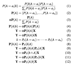
Because of the scaling factor α, we can multiply the right-hand-side of the equation by any non-zero constant k (6).

In equations (7) and (8), we introduce our “flat world” assumption F, where all values of P(A) are equally likely. Note that any conditional probability that fixes that value of A is unchanged under this assumption (8). Substituting, we get equation (9), and do the usual conditional probability shuffle (10-11). We can then allow α to re-absorb a constant factor, giving us the rule we need to justify applyProb (12).

The final classifier

Now we’re ready to put it all together. A classifier can be represented as a score and a vector of probabilities:

data Classifier = Classifier Double [Prob]
  deriving Show

classifier f =
  Classifier (score f) (classifierProbs f)

applyClassifier (Classifier _ probs) =
  applyProbs probs

Using these tools, we can write:

> classifier (hasWord "free")
Classifier 0.23 [84.1%,15.9%]

We also want to sort classifiers by score:

instance Eq Classifier where
  (Classifier s1 _) == (Classifier s2 _) =
      s1 == s2

instance Ord Classifier where
  compare (Classifier s1 _)
          (Classifier s2 _) =
    compare s2 s1

Now we can turn our table of word counts into a table of classifiers:

classifiers :: M.Map String Classifier
classifiers =
    M.mapWithKey toClassifier wordCountTable
  where toClassifier w _ =
          classifier (hasWord w)

findClassifier :: String -> Maybe Classifier
findClassifier w = M.lookup w classifiers

Given a list of words ws, we can look up the n classifiers with the highest score:

findClassifiers n ws = 
    take n (sort classifiers)
  where classifiers =
          catMaybes (map findClassifier ws)

We can now rewrite hasWords as a simple fold, incorporating all our tweaks. Here’s the heart of Paul Graham’s Plan for Spam:

hasWords' ws prior =
  foldr applyClassifier
        prior
        (findClassifiers 15 ws)

And we’re in business:

> bayes (hasWords' ["bayes", "free"]
                   msgTypePrior)
[Perhaps Spam 34.7%, Perhaps Ham 65.3%]

Note that this final design could be trivially ported to C++ and tuned for maximum performance. See Norvig’s lecture for a discussion of how to store probabilities efficiently—Google gets by with as few as 4 bits for some applications.