Robot localization using a particle system monad

Refactoring Probability Distributions: part 1, part 2, part 3, part 4, part 5

Welcome to the 5th (and final) installment of Refactoring Probability Distributions! Today, let’s begin with an example from Bayesian Filters for Location Estimation (PDF), an excellent paper by Fox and colleagues.

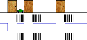
In their example, we have a robot in a hallway with 3 doors. Unfortunately, we don’t know where in the hallway the robot is located:

Robot at
first door

The vertical black lines are “particles.” Each particle represents a possible location of our robot, chosen at random along the hallway. At first, our particles are spread along the entire hallway (the top row of black lines). Each particle begins life with a weight of 100%, represented by the height of the black line.

Now imagine that our robot has a “door sensor,” which currently tells us that we’re in front of a door. This allows us to rule out any particle which is located between doors.

So we multiply the weight of each particle by 100% (if it’s in front of a door) or 0% (if it’s between doors), which gives us the lower row of particles. If our sensor was less accurate, we might use 90% and 10%, respectively.

What would this example look like in Haskell? We could build a giant list of particles (with weights), but that would require us to do a lot of bookkeeping by hand. Instead, we use a monad to hide all the details, allowing us to work with a single particle at a time.

localizeRobot :: WPS Int
localizeRobot = do
  -- Pick a random starting location.
  -- This will be our first particle.
  pos1 <- uniform [0..299]
  -- We know we're at a door.  Particles
  -- in front of a door get a weight of
  -- 100%, others get 0%.
  if doorAtPosition pos1
    then weight 1
    else weight 0
  -- ...

What happens if our robot drives forward?

Driving down the hall

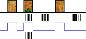
When our robot drives forward, we need to move our particles the same amount:

Robot at
second door

This time, we don’t detect a door, so we need to invert our blue line. Once again, this allows us to filter our some particles.

In Haskell, we would write:

localizeRobot = do
  -- ...
  -- Drive forward a bit.
  let pos2 = pos1 + 28
  -- We know we're not at a door.
  if not (doorAtPosition pos2)
    then weight 1
    else weight 0
  -- ...

The next time we move, things start to get really interesting:

Robot at
third door

We can rule out all but one clump of particles! In Haskell:

localizeRobot = do
  -- ...
  -- Drive forward some more.
  let pos3 = pos2 + 28
  if doorAtPosition pos3
    then weight 1
    else weight 0
  -- Our final hypothesis.
  return pos3

And that’s it! We can run our particle system as follows:

> runWPS' localizeRobot 10
[97,109,93]

In this example, we run our particle system with 10 particles, 3 of which survive the whole way to the end. These are clustered about 1/3rd of the way down the hallway, giving us a pretty good idea of where we are.

Unweighted Particle System Monad

OK, so how does our monad work? This gets pretty technical, so you may want to review part 1 and part 2 before continuing. Alternatively, you could just scroll down to the last section.

To begin with, let’s ignore the weights. We can represent a particle system as function that maps an integer to a random list of particles:

newtype PS a = PS { runPS :: Int -> Rand [a] }

The integer tells us how many particles to return:

> runRand (runPS (uniform [1..10]) 5)
[3,2,9,5,10]

If we have a random value of type Rand a, we can build a particle system of type PS a by sampling that random value repeatedly. Building on the code from part 2, we get:

liftRand :: Rand a -> PS a
liftRand r = PS (sample r)

Given a particle system of type PS a, and a function of type a -> b, we can construct a particle system of type PS b by running the particle system and applying our function to each particle:

instance Functor PS where
  fmap f ps = PS mapped
    where mapped n =
            liftM (map f) (runPS ps n)

We also need to define the monadic return and >>= operators. The former can be built from return operator for Rand:

instance Monad PS where
  return = liftRand . return
  ps >>= f = joinPS (fmap f ps)

As for the latter, it’s usually easiest to define >>= in terms of a join operation. And join is where the magic happens—we need to collapse a value of type PS (PS a) into a value of type PS a:

joinPS :: PS (PS a) -> PS a
joinPS psps = PS (joinPS' psps)

joinPS' :: PS (PS a) -> Int -> Rand [a]
joinPS' psps n = do
    pss <- (runPS psps n)
    xs <- sequence (map sample1 pss)
    return (concat xs)
  where sample1 ps = runPS ps 1

The code is a little tricky, but the basic idea is simple: We run our outer particle system, producing n particles. But each of these particles is itself a particle system, which we run to produce a single particle. We then combine the n single-particle results into one result with n particles.

We also need to make our particle system a probability monad. Again, we can do this by reusing code from Rand:

instance Dist PS where
  weighted = liftRand . weighted

Note that this monad isn’t ready for production use—it’s still pretty slow, and it doesn’t give us any way to access our sensors.

Weighted Particle System Monad

The weighted version of the particle system is a bit easier. We can just reuse PerhapsT, which transforms an existing monad into one with a per-element weight:

type WPS = PerhapsT PS

We also need to make WPS into a probability distribution:

instance Dist (PerhapsT PS) where
  weighted = PerhapsT . weighted . map liftWeighted
    where liftWeighted (x,w) = (Perhaps x 1,w)

Next, we need a way to update the weight of a given particle. Note that this is closely related to applyProb from part 4.

weight :: Prob -> WPS ()
weight p = PerhapsT (return (Perhaps () p))

Finally, we need a way run a weighted particle system:

runWPS wps n = runPS (runPerhapsT wps) n

In our example, we also use a wrapper function to clean up the output a bit:

runWPS' wps n =
  (runRand . liftM catPossible) (runWPS wps n)

catPossible (ph:phs) | impossible ph =
  catPossible phs
catPossible (Perhaps x p:phs) =
  x:(catPossible phs)
catPossible [] = []

You can download the latest version of this code using Darcs:

darcs get http://www.randomhacks.net/darcs/probability

In a more sophisticated implementation, we’d want to periodically resample our particles, discarding the ones with weights near zero, and increasing the number of particles near likely locations.

More cool stuff

Bayesian Filters for Location Estimation (PDF) is an excellent (and very accessible) overview of belief functions. If you’re into robotics or probability, it’s definitely worth checking out.

As sigfpe points out, PerhapsT is closely related m-sets, which turn up a lot whenever you’re working with matrices. In fact, you can build a monad from any measure space, including possibility and other models of beliefs.

Don’t miss sigfpe’s excellent articles on quantum mechanics. He shows how to generalize the probability monad to support quantum amplitudes and mixed states.

Given all this cool stuff, I strongly suspect that monads are the Right Way to represent probability and beliefs in programming languages.

Dan P wrote on Apr 20, 2007:

I haven't fully read this yet but does this approach must have any relationship with the Viterbi algorithm? I'm writing a blog entry on Viterbi and this stuff looks remarkably similar.

Eric wrote on Apr 21, 2007:

I'm looking forward to your blog post! I don't know much about the Viterbi algorithm. Particle systems are similar to random sampling, except that the samples are taken "in parallel" instead of one at a time. This offers two advantages: 1) You can maintain a series of hypotheses about the world, and update them as new evidence arrives. This is especially handy in robotics. 2) You can periodically reallocate your particles towards the most promising hypotheses. This is very handy in long-running computations where a large fraction of hypotheses are ruled out at each step. I've seen nice 2D movies of particle systems, which make these ideas very intuitive. I'll have to see if I can dig one up.

Noel Welsh wrote on Apr 23, 2007:

Particle filters and the Viterbi algorithm are used in similar situations. The Viterbi algorithm is typically used to calculate the most likely transitions through a model given observations when the state space is discrete. Particle filters are typically used to calculate a set of high probability transitions when the state space is continuous, and not of an easily analysable form (so a Kalman filter cannot be used).

Christopher Tay wrote on Apr 23, 2007:

I would like to first say that although I do not program haskell, I really enjoy your blog :) Some points I would like to add... A particle filter is essentially monte carlo (sampling). It is also known as markov chain monte carlo (MCMC). The particles are samples which represents a certain probability distribution which in this case, represents the state space of the robot. Essentially, the set of particles gives us an approximation of the probability distribution on the state of the robot. Its advantage over the kalman filter are essentially its non linearity (of robot state transitions in this case) and its ability to represent multi-modal distributions (which is not the case for kalman where it is assumed to be gaussian). In contrast, the viterbi algorithm frequently associated with hidden markov models estimates not the probability distribution, but rather the most likely solution. The application of the two methods are not limited by whether the state space is continuous or discret (although it does often have practical implications). Both the viterbi algorithm and particle filters can be applied to discrete and continuous spaces.

Eric wrote on Apr 23, 2007:

Noel & Christopher: Thanks for comments! Kalman filters, AFAICT, are one of the few models of belief functions that don't map cleanly to Haskell monads. So far, I haven't been able to define a suitable version of fmap. One especially cool thing about particle systems is that you can use a GPU to simulate a million particles in real-time. Given the handy monadic structure of particle systems—and their ability to represent non-linear functions--it's worth keeping particle systems in mind. With the right hardware, they're fast, flexible and easy to program.

Samer Abdallah wrote on May 21, 2007:

I've been playing with sampling monads and I've run up against a problem which I believe will afflict this code as well. The problem comes up when we add a conditioning operator, or equivalently, if we allow an mzero into the monad. A trivial example might be something like > y = do u <- uniform01; guard (u>=0.5); return u or, in my code > y = cond (>=0.5) uniform01 this is a (not particularly good) way of sampling uniformly on [0.5,1), but you get the idea. If we now elaborate this to > z = uniform01 >>= \u->cond (>=2u) uniform01 or > z = do u <- uniform01; v <- uniform01; guard (v>=2u); return v we get something where, if the first sampling returns u>=0.5, the guard on the second sample cannot succeed. A naive sampling method which tries to repeat the second sampling operation until the guard succeeds will get stuck in an inifite loop, as there is no way for it to realise that its task is hopeless and it needs to backtrack and retry the first sampling operation. In your code, the sample problem would occur when calling |sample1 x| if x cannot return any samples (due to guards being present in the definition of x). As I see it, I can think of two ways around this. One is to supplement the representation of the random variable to include sufficient static information about the support of the distribution so that cond can immediately reduce to mzero if the conditioning event (ie a set) does not intersect with the support. The other is to have the representation be a stream of |Maybe a| and implement a kind of 'fair' binding in x >>= f (or equivalently a 'fair' join) which *interleaves* the stream of samples from each application of f to samples from x. That way, if x returns [x1,x2,...], and guards make |f x1| a stream of |Nothing|, then at some point, we will get to try |f x2|, |f x3| and so on. This is the same as the 'fair conjuction' proposed by Shan et al in their LogicT monad (see http://okmij.org/ftp/Computation/monads.html). I'm just trying it now but looks like it's going to be very inefficient because it can waste a lot of samples and suffers from combinatorial explosion when you start tupling up random variables. Have you come up against this problem and do you have any thoughts on the matter?

Eric wrote on May 25, 2007:

Adding mzero to a probability monad has tricky semantics. In the particle system above, I keep the "impossible" particles and give them a weight of 0. In a real implementation, you would generally want to replace these particles by "spliting" high-probability particles in half, or by resampling the particles periodically, resetting all the weights to 1. In an earlier hack I used the "missing probability" to represent the normalization factor needed by Bayes' rule. It's important to understand exactly how guard fits into your larger semantics; there are quite a few traps for the unwary. At a minimum, if you're going to build a sampling-based probability monad with an mzero, you're going to have to make sure that sample 200 (guard False) immediately returns zero samples.

chris wrote on Aug 02, 2007:

Christopher, you are wrong. A particle filter is not a markov chain monte carlo (MCMC) algorithm. A MCMC algorithm is an iterative algorithm and is used for batch tasks. Particle filters only rely on importance sampling and resampling mechanisms and allow you to address sequential problems.

Christopher Tay wrote on Sep 06, 2007:

Chris, you're right. Its sequential monte carlo. Thanks for pointing it out.

Driving down the hall

Unweighted Particle System Monad

Weighted Particle System Monad

More cool stuff

More posts